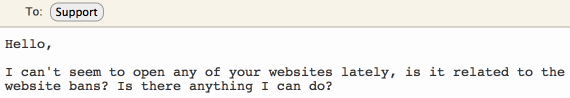
or how you can get from this:

to this:

This is a fairly long read, so I split it into a number of bigger sections:

1. Intro
2. Collecting data
3. Processing data
4. Visualising data
5. Conclusions

Full code for the project is available in morhekil/nutprobe repository on GitHub, and the visualisation is available on Tableau Public as Domain Availability worksheet (you can download its source code there, too).

Intro

Back story

One of my clients is an online gaming company, that runs online poker, casino and betting website. Not that long ago, Russian government decided to start actively blocking online resources it doesn’t like for various reasons, and plenty of online poker websites got smashed by that ban hammer – as poker is currently constrained to a limited gambling areas only in Russia.

This led to a serious loss of players for that client of mine, as the company was working with the Russian market only – so we had to pivot a bit, but we also wanted to understand just how bad the situation is. How to do it? Well, as I’m going to show you – just deploy some client-side tracking, collect and summarise the data, and visualise the result to create an easy-to-understand picture.

The task

Ok, so let’s begin by more or less formalising the task. We have a number of domains, and we need to find out which of them are available to our users, and which are blocked by the ISP. The data should be collected over time, and preferably – split by user’s geographical location, and even his ISP, to let us see the effects of either our evasive maneuvers, or ISP config changes.

As this is not a production-critical feature, but rather an experiment in curiousity (from my side), or in gaining some insight (from client’s side), it does not have to be particularly high performant, or even optimal at all. Doesn’t sound like much of a challenge, does it? Ok, let’s add some contraints!

The constraints

To make this whole study a more interesting exercise, let’s enforce on ourselves the following set of constraints:

1. Let’s build a general-use tool, that does not require any custom server-side infrastructure from its user. Free third-party services are a fair game, though.

2. As a corollary of the previous constraint, data collection should happen directly client-to-storage. This basically requires data processing and analysis to happen out-of-band, at some later stage.

With that in mind, let’s see what we can use to build it.

Toolset

The first constraint is probably the more interesting one. What could be used to accepts data directly from users’ browsers? My first reaction would be to spin up Redis with some web API in front of it (say, just barebones Webdis), but it violates “no custom infrastructure” requirement.

What else? Well, there’s that Firebase thing, that promises all and everyone an awesome data backend and API. Sounds good enough, let’s take it for a spin.

Client-side data collection will, of course, have to use Javascript. And you know what? Given that Firebase provides an NPM package, let’s go crazy and write data processing in Node.js, too. Yeah, yeah, I know, Node.js is cancer and all that, but we’ll all be cured eventually.

And the last piece is data visualisation. As a proof of concept, and in the name of keeping things simple – let’s not write more code for it, but rather use an existing platform for data vis, that is Tableau Public. While the commercial Tableau Server is fairly expensive, Public edition is just good enough for our needs.

Collecting data

Firebase setup

With the introduction out of the way, let’s start on the first part of the task. And the first thing to be done – Firebase database setup. There’s really only one thing to set up – access controls. After some consideration and a few experiments, I ended up with the following:

1. A top-level node contains a list of all received reports, and it is available write-only for all clients – so anyone can write there, but can’t read back.

2. For authenticated clients (e.g. the data processor), it is also available for reads to consume the reports. All other nodes are read/write for authenticated clients.

The is implemented by the following security rules:

{
    "rules": {
        ".read": "auth != null",
        ".write": "auth != null",

        "reports": {
          ".write": true
        }
    }
}

Client side probe

We have a place to write data to now, but what do we write? Well, we need to know what we tested (domain), the result of the testing (success/failure), ip of the client, and the timestamp of the report.

To check the domain, let’s simply pull a known URL off it, that is known to exist and returns a response as small as possible – e.g. an empty gif, a really small page, etc. If target is the parameter with the value of the URL to check, and logResult – function that logs the result, the check function could look like this:

// Entry point for a target check. Fires off a request to the given target,
// and logs the result
var check = function(target) {
  try {
    j.request('GET', target).then(
      function(res) {
        if (res !== expected) { logResult(target, false, res); }
        else { logResult(target, true); }
      },
      function(xhr) {
        logResult(target, false, (xhr.status + ' ' + xhr.statusText).trim());
      }
    );
  } catch(error) { logResult(target, false, error); }
};

If you’re curious about that then call – this is a promise, implemented on top of a lightweight RSVP.Promise library here. I’m using promises quite heavily throughout the code, but if you’re not familiar with the concept – you can think of them as “delayed” value, which resolve when the data they represent is ready.

Alright, what’s next? To put together the full report, we need to know client’s own ip address. And it needs to be an external one – as users are behind NATs, and we need their real public IP. While there are various ways to do it, the simplest one to execute from a browser is probably to use JSON API from HostIP.info. If you click on that link, you’ll see a JSON response with your IP address, and some basic GEO lookup data, and that IP address is what we’re after. So the IP lookup function comes out as:

// Get IP of the current machine via HostIP API.
// Returns memoized promise, that resolves with the IP address string.
// Memoization allows to query HostIP API only once per page load, avoiding
// unnecessary extra requests transparently to function's clients.
var getIP = function() {
  var ip_promise = null;

  return function() {
    if (ip_promise === null) {
      ip_promise = new RSVP.Promise(function(resolve, reject) {
        j.json('GET', 'http://api.hostip.info/get_json.php').then(
          function(hostip) { resolve(hostip.ip); }
        );
      });
    }
    return ip_promise;
  };
}();

Looks like we have all we need. Now the final step – report it to Firebase. This is easy – we just need to get the Firebase client connected, and send up the data hash:

// Log status of the given target into Firebase.
// Adds current timestamps to the report data, and an optional message string
var logResult = function(target, status, msg) {
  RSVP.hash({
    firebase: getFirebase(),
    ip: getIP()
  }).then(function(r) {
    var fbref = new Firebase(fbUrl);
    var report = {
      target: target,
      ip: r.ip,
      success: status,
      message: msg || '',
      created_at: (new Date()).toISOString()
    };
    fbref.push(report);
  });
};

This function is also responsible for chaning together Firebase connection and IP address lookup, to parallelize them, and to send the report when both are ready – RSVP.hash is resolved when all of its members are resolved.

And that’s it! Once everything is put together (and you can see the final code on GitHub), it can be deployed via user-facing website pages using an html snippet like this one:

  <script src="/probe.static.js" type="text/javascript"></script>
  <script type="text/javascript">
    try {
      var nutprobe = require('nutprobe/probe').default;
      var targets = [
        '//domain1.com/ping',
        '//domain2.com/ping',
        '//domain3.com/ping'
      ];
      var expected_answer = 'pong';
      var report_success = true;
      var cooldown_days = 1;
      nutprobe(targets, expected_answer,
               'https://yourname.firebaseio.com/reports',
               report_success, cooldown_days);
    } catch(e) {};
  </script>

When this is deployed, you should quickly see the reports like this one start popping up in your Firebase instance:

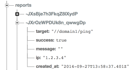
Leave the reports to accumulate for a while, and let’s move on.

Processing data

Now that we have the required data with the reports in Firebase, it is time to start processing them. There are, of course, many ways to skin this particular cat, but I have two considerations:

1. The processed data has to be reasonable human-friendly, and provide some insight even without a visualisation layer, or server as a debugging tool for data vis issues.

2. But still, the data will be fed into a visualisation engine, so it needs to play well there.

With all that in mind, this is the summarised data structure I came up with:

1. Reports are summarised into a tree of the following structure:

• Date
  • Target domain
    • Country
      • ISP
      • City
        • ISP

2. On every level of that tree after the “target domain” one, two nodes are added – “succ”, and “fail”, those contain success and failure counters for the whole subtree.

This structure allows to quick see the overall availability of the domains even with a naked eye – say, if I want to see how well my “domain1” performed in “Russia” on September 29th, I just open 20140709 → domain1 → Russia, and look at the value of “succ” and “fail” nodes. And for visualisation we’ll dig all the way down to the leaves.

Now, what are we going to do with our data? The processing steps are as follows, for every report received:

1. Look up geographical information for the reported IP address. 2. Based on this information, and the outcome (whether the domain was available or not), increment appropriate succ/fail counters at all nodes of the tree corresponding to the ISP and its location. 3. Remove the report data from Firebase.

Simple enough, let’s start.

Geo lookup

And, actually, I have to confess – this is the part where I had to break “free tools only” requirement, and relax it to “cheap tools”. Unfortunately, after some digging online, I couldn’t find a service (or even just a publicly available database) that would allow me to lookup an ip address geo data down to its ISP name. And whois is an ungodly mess these days. So in the end, I ended up using GeoIP2 Precision Services from Maxmin, that is a fairly cheap ip geo lookup service. $20 will give you 50,000 queries, which is more than enough for my needs.

To keep the costs down even more, it might be a good idea to keep a cache of IP lookups somewhere else, to avoid doing querying Maxmin for the same IP again and again. And, as we already have Firebase – let’s just use that as a cache layer.

I’m not going up to copy the full code here, as there’s a certain amount of boilerplate and error handling that is not really interesting, but using geoip2ws NPM module the actual lookup can be done as easily as this:

var geo = require('geoip2ws')(process.env.MAXMIND_UID, process.env.MAXMIND_KEY),
    Q = require('q');

// Query Maxmind web service for geo location data
function queryMaxmind(lookup) {
  var dfr = Q.defer();
  geo(lookup.ip, function(err, geodata) {
    if (err) { dfr.reject(err); }
    else { dfr.resolve(geodata); }
  });
  return dfr.promise;
}

Here I’m using promises again to handle asynchronous execution, but as this is now a server-side code – I’m using more feature-rich Q Promise rather than the previous lightweight RSVP.Promise.

Full lookup is based on two chained promises – read the cache first, and fall back to Maxmind lookup if nothing is found in the cache. Promises allow to implement it beautifully:

// Main API - perform a lookup of the given IP address.
// It checks local and Firebase caches first, and if the IP information is not
// there - queries Maxmind, and writes the value into the Firebase cache
ipgeo.lookup = function(ip) {
  return Q.Promise(function(resolve, reject) {
    readCache(ip)
    .then(queryMaxmind)
    .then(resolve, reject)
    .done();
  });
}

I won’t go into full details of readCache here, but you can read the full source code on GitHub, and ask questions in the comments if you have any. The only notable mention is the Firebase cache format – I’m writing full response from Maxmind into the cache, so that every record looks like this:

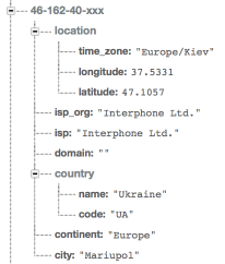
Just keep this structure in mind – it will come in handy, when we start visualising this data.

Writing counters

With all required data now available, the next is to write summarised counter values at all requires nodes of the statistics tree. The naive way would be to do the standard read-increment-write loop, but as you might have guessed - this is not really going to work. Why? Because if there’re multiple write operations happening at the same time, it will lead to a classical race condition, with one operation overwrite the increment value just saved by another operation.

Thankfully, Firebase provides native support for transactions, so there’s no need to resort to external mutexes, or other concurrency controls. Let’s wrap this operation into a function, that takes an array of nodes representing the path in the tree, and success/failure flag, and transactionally increments the appropriate counter under the given path:

// Transactionally writes a single success/failure atom into the statistical
// data. Returns a promise that resolves with the data write is confirmed.
function writeTick(keys, success) {
  var dfr = Q.defer();

  var key = keys.map(function(key) { return key.replace(/\W+/g, '-') }).join('/');
  var ref = new Firebase(
    [ process.env.FBIO_STATS_URL, key, success ? 'succ' : 'fail' ].join('/')
  );
  ref.transaction(
    function(val) { return val*1 + 1; },
    function(err) { err ? dfr.reject() : dfr.resolve() }
  );

  return dfr.promise;
}

ref.transaction here is that Firebase API call to modify the data transactionally. Note that the promise is returned – as we’ll need to increment multiple counters for every received report, we can use a feature of promises that allows to convert an array of promises to a single overarching promise, and just wait until this final promise is resolved – it will indicate that all underlying operations have been completed:

// Write full set of summarised statistics derive from the given report data
// and the related geo location.
function writeStat(report, geo) {
  var date = report.created_at.split('T')[0];
  var workers = [
    [date, report.target],
    [date, report.target, geo.country.code],
    [date, report.target, geo.country.code, 'ISP', geo.isp],
    [date, report.target, geo.country.code, 'CITY', geo.city],
    [date, report.target, geo.country.code, 'CITY', geo.city, geo.isp],
  ].map(function(keys) {
    return writeTick(keys, report.success);
  });

  // return an all-promise, that will resolve when all promises returned by
  // writeTick are resolved.
  return Q.all(workers);
}

The main processing loop then becomes essentially a chain of write-cleanup operations, sans the errors handling:

// Process a report item, given its id and the data reported
function processItem(rid, report) {
  var dfr = Q.defer();

  ipgeo.lookup(report.ip)
  .then(function(geo) { return writeStat(report, geo); })
  .then(function() { return cleanupItem(rid); })
  .then(function() { dfr.resolve(); })
  .fail(function(err) { dfr.reject(err); });

  return dfr.promise;
}

Other operations (cleanup, etc) are fairly trivial, and the full code is here on GitHub

Wrapping it up

And it is essentially all there is to processing. All that’s left is to wrap it into a runner function, that will load report data from Firebase and pass it down into for processing – this is implemented in a naive way by this module.

When I’m saying “naive” here, I mean the fact that the processing is done is small batches, which is fairly slow – if I were to take it to the full production scale, I would replace it with handling out this work to a number of workers for faster processing, but it seems to be an unnecessary complexity for this small-scale experiment.

Visualising data

Now to the final step – presenting all these numbers in a nice and human-friendly way. Tableau Public can not connect directly to any APIs or services, but it can accept a plain old CSV file – so let’s generate one. For Tableau there’s no need to worry about summarising the data, etc – all of that can be done inside Tableau itself, so it is usually much better to give Tableau access to a fine-grained data, to have more detailed material to work with.

Exporting summarised data

Exporting the data itself is quite easy – as we know the depth of the tree in advance, we can approach with a naive recursive depth-first traversal, and just print out the part in the tree once we have reached a leaf at the given depth.

And thinking a bit ahead, in Tableau we’ll want to visualise not just a number of successful or failed checks, but rather the proportion of failures – so let’s precalculate this value as we’re traversing the tree, as well as the total number of hits we have for the node.

The recursive tree traversal is easy enough to implement:

// Recursively export tree under the given root, optionally filtering nodes
// according to the given function
function exportTree(root, tree, parents) {
  var filter;
  if (!parents) { parents = []; }

  if (!tree || typeof(tree) != 'object') {
    // reached a leaf - print the whole branch
    printBranch(parents.concat([root, tree]));
    return;
  }
  // Calculate failure rate, of either succ or fail counter is present at
  // this node
  if (tree.succ || tree.fail) { calcRate(tree); }
  // Reset parents history at the given tree depth
  if (parents.length == treecfg.targets_at) { root = treecfg.targets[root] || root; }

  Object.keys(tree).map(function(node) {
    exportTree(node, tree[node], parents.concat([root]))
  });
  return true;
}

And that prentBranch function actually prints only the branches at the depth at or more than the configured one:

// Prints out given branch
function printBranch(nodes) {
  if (nodes.length >= treecfg.mindepth) {
    // node is at the required depth - this is the data we're interested in,
    // print the branch
    console.log(nodes.join(','));
  }
}

The rest of the helper functions are trivial, and you can find them all in the full source code".

When the exporter runs, it generates a csv data similar to this sample:

Date,Domain,Country,X,City,ISP,Hits,FailRate
2014-09-27,Poker RU Main,RU,CITY,Moscow,Limited-Liability-Company-Expaero,1,0
2014-09-27,Poker RU Main,RU,CITY,Moscow,MTS-OJSC,2,0
2014-09-27,Poker RU Main,RU,CITY,Moscow,OJS-Moscow-city-telephone-network,4,0
2014-09-27,Poker RU Main,RU,CITY,Moscow,OJSC-Central-telegraph,2,0
2014-09-27,Poker RU Main,RU,CITY,Moscow,OJSC-Rostelecom,9,0

And it’s almost perfect, except for one problem – if you import this data into Tableau, and try to display it on a world map, you won’t see much – Tableau doesn’t know that many cities outside of US, and it will have a hard time finding a corresponding geographical coordinates for, say, Barnaul in the middle of Siberia. We’ll need to help it with that.

Exporting location longitude and latitude

This is where cached geo data that we haved build for Maxmind lookups comes in very handly. It already contains the full list of cities with their geo coordinates, just grouped by IP – so let’s reprocess it, and convert it into a flat list of locations and their coordinates instead. All we need for that is to loop over the list of caches, and print out new locations as they appear:

var cities = { NA: true };

// Export received snapshot as csv data
function exportData(snap) {
  process.stdout.write("City,Latitude,Longitude\n");
  snap.forEach(exportNode);
}

// Export data from the given node
function exportNode(node) {
  var val = node.val();
  if (!cities[val.city]) {
    cities[val.city] = true;
    process.stdout.write([
      val.city.replace(/ /g, '-'), val.location.latitude, val.location.longitude
    ].join(',') + "\n");
  }
}

This should print out locations nicely in the following form:

City,Latitude,Longitude
Taipei,25.0392,121.525
New-York,40.7267,-73.9981
Vinnytsya,49.2328,28.481
Tula,54.2021,37.6443
Omsk,55,73.4
Tomsk,56.5,84.9667

And with these two files generated, we’re all set to build the final visualisation.

Building the visualisation

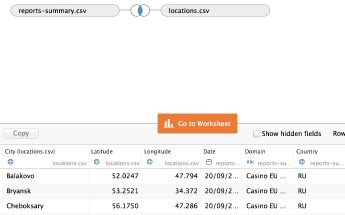
As the first step, let’s import the data into Tableau. Just adding the files to the worksheet is enough – as the data columns are named appropriately (City, etc), Tableau is smart enough to recognise relationships between the data, and automatically associate city names with the appopriate geo location data from the second file. The data should look like this:

Let’s move onto the worksheet itself. First, we’ll need another calculated field that contains both city and ISP name together – just click on any column, select “Create Calculated Field”, and enter a simple string concatenation as [City]+", "+[ISP], and give it a name – say, City and ISP.

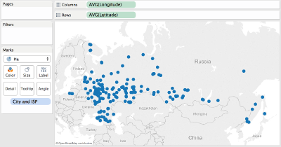
When this is done, time to arrange the data. Start by dragging Longitude and Latitude into Columns and Rows, followed by City and ISP going into “Marks” block. This should result in a nice map like this one showing up:

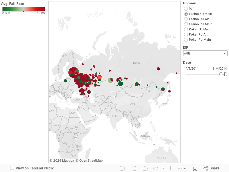
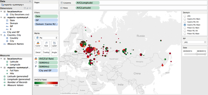
Now, let’s set up a better representation of failed and successful check rates. Let’s display each city as a pie chart, with its size proportional to the total number of hits received from this city – we should see Moscow as the biggest marker, followed by Saint-Petersburg, etc. Each slice on the pie chart should represent a specific ISP, and its color is proportional to the failure rate - from green being 0 (no failures), to red being 1 (all checks from this city and this ISP have failed).

This probably took longer to read (or write), than it will take you to actually configure the visualisation. Step by step:

1. Start by changing mark type from “Automatic” to “Pie”
2. Drag Hits column from the summary report data on to “Size” and “Angle” targets.
3. Drag Failrate from the same on to “Color” target.
4. Double-click on the gradient bar, and change it to Red-Green reverse gradient.

Now, as the last touch, let’s set up some filters – e.g. add Domain as a single value list filter, add Date as a data range filter, and ISP as a single value dropdown filter. The final result should resemble this picture:

And voila – that’s it! Now even the most non-technical person can easily pull up this report, and dig into the data as deep as it allows. And that I believe to be the most important result – not just to collect the data, but also to make it easily available to any human being.

Conclusions

As this was an experiment, let’s draw some conclusions about what has been done, and a various tech used in the process.

Firebase

Firebase worked well as a simple data storage. Will I use it for a production project in the future? Unlikely, but it looks like a great fit for small experiments or hackatons.

I’d probably like to see more database-grade features in it first, before even considering moving important data on it – e.g. data snapshots/backups as the first thing that jumps to mind.

No-custom-server approach

Suprising, also worked well. It appears to be completely possible to build complete solutions to various software problems without any custom server side pieces, using only publicly available third-part technologies.

Tableau

Tableau is awesome for quick proof-of-concept visualisations, those can be easily uploaded online and shared with others. Sometimes its visualisation capabilities are quite limited, so if your business depends on data visualisation as its cornerstone – I’d still consider investing into building a more capable data visualisation using technologies such as D3.js.

But if visualisation is just another tool for your project – then it is quite likely that Tableau will fit just right.

Thank you

If you’re still reading at this point – I’m very grateful, and would like to thank you for your attention. I’m sure you have questions, as I was quite brief in this post – feel free to ask any of them in the comments below.